Anarchies Crossover Design

Integrating the Drivers

Crossover Goals

This design is intended to be my best work and the centerpiece of my main listening spot in my home for the foreseeable future.  To meet that goal while not spending time and money doing trial and error prototypes it’s critical to do as accurate of a simulation as possible.  To do that, the simulation tools have to have as accurate data for the input as possible.

Previous design work has been using tools such as those built in Excel, WinPCD and Xsim.  These tools tend to focus on a single point design, typically on axis and 1M away.  This design work is great for a near field studio monitor where you’ll actually be listening to them at about 1M away but doesn’t really represent how a typical HiFi setup will be utilized in a larger room and at a greater distance.  For these situations the total energy output to the room considering all directions needs to be determined for the best results.  The power response is exactly that measurement, and a simulation of this during crossover design is important for the final results in a room.

Enter Vituix CAD

A relatively recent addition to the speaker design software available is Vituix CAD, a one stop shop of tools that can do many of the tasks previously described in my earlier article Advanced Speaker Design Simulation. Vituix includes tools that will:

• Model woofers in enclosures
• Model diffraction effects from the baffle
• Merge near and far field measurements, with baffle effects
• Output files in minimum phase, or just calculate them on the fly in the simulation
• Calculate basic room reflections
• Process raw impulse measurement data with detailed time gate and advanced FFT parameters

Additionally, the simulation can use multiple off axis measurements and calculate actual power response for the speaker at different listening distances.

The software itself is free, and the support is worth every penny!  That is to say, the documentation is very complete, but not necessarily written for the layman.  Your best bet may be to join in some discussion online to solicit some help from experts.  I have a fairly advanced understanding of the methods here but lack some of the advanced math skills to understand some of the why behind the impulse data, FFT conversion and gating, and other advanced calculations going on.  Ultimately I needed help here as well, and remain far from an expert on this process but will do my best to explain what I learned in the process here.

Gathering Data

You can’t start a design without the proper raw measurements of the speaker in real life.  Well… you can given good quality OEM measurements and models of the cabinet for woofer loading, baffle step and diffraction effects but those will always be guestimates.  The best method will be to get your measurements in the actual cabinet with the actual speakers you’re building.

My previous work has been using the very affordable iMM6 microphone from Dayton Audio plugged into my trusty Surface tablet.  That gets you a decently accurate microphone accessible to proper measurement programs.  The details of the process were written up in my Supernova Minimus design, and the results of that speaker were excellent.  The main downside of the iMM6 is the placement, which is 100% dependent on where you can place the tablet or laptop.  Using a basic music stand, the far field measurements were fine, but close mic measurements within a couple mm of the cone are difficult to do while just holding the tablet by hand.  For a bit more of an investment, I acquired another Dayton Audio mic, the EMM6.  This is a phantom powered XLR connected mic for any computer using a proper studio audio interface.  Many folks will need to get one of those too, and many are available for home studio or podcasting use at reasonable costs.  I happen to have a recording setup already with 12 channels of input ready to go between a Focusrite Scarlett interface extended by a Behringer 8 channel ADAT interface pre-amp.  For that reason the decision to go with an XLR mic was really easy.  Here’s the most important point to consider:

The iMM6 as well as any USB connected measurement mic will always be limited to single channel measurements.

This is a limitation for design for one important reason:  There is no timing reference data to determine when the signal was sent to the speaker compared to when the sound arrived at the microphone.  This limits your simulation data and forces you to manually determine the acoustic offsets between your drivers and process everything with minimum phase.

Timing between drivers

This is critical for simulation!  Sound travels at a finite speed, and small differences in distance between the speaker and the microphone will add phase to the signal, drastically altering how it will add to another speaker near it at the same frequency.  This is all based on wavelength of the sound in the air, so the higher the frequency the shorter the wavelength, thus the delay introduced with small changes in distance equate to larger phase angle changes.

2 Channel Measurement

By using feedback of the electrical signal going to the speaker, the measurement software knows exactly how much time passed before the sound arrived at the microphone, and therefore the measurements of each speaker will be phase accurate at the measurement point without any summing and comparison.

There are several levels of 2 channel measurements, and a whole lot more technical detail of what is happening.  Frankly, I barely understand that myself so for additional information check out the user manual, message boards and prepare to spend some time doing the googles.

Spinorama

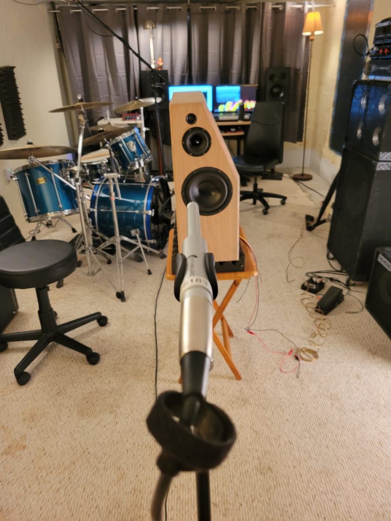
In order to simulate and show the full power response of your design in Vituix, a whole lot of off axis data is best to get the data on what is really happening.  Some folks build fancy turntables with calibrated marks every 10 degrees, and those folks usually also have a bit better space to actually execute those measurements.  In my case, the measurement space is small with under 7 feet the maximum I can get to any boundary.  I also didn’t want to invest in a turntable quite yet, so I opted for measurements only every 15 degrees, roughly calibrated with painter’s tape on the floor and an eyeball alignment to keep the face of the baffle at the same origin.

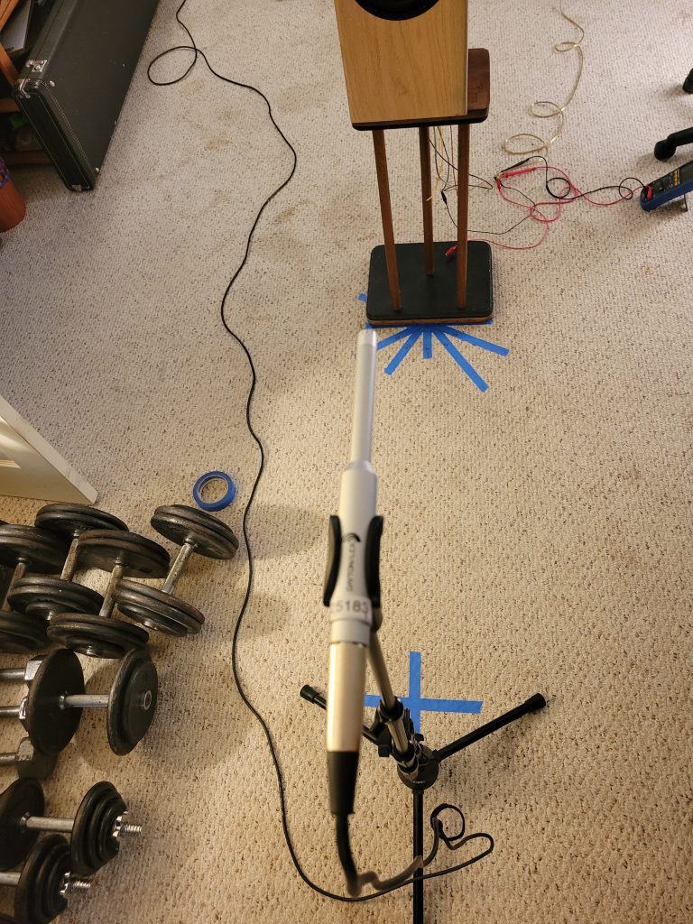
Using ARTA, I followed the measurement guide for Vituix as closely as possible.  I setup the normal semi-dual connection with the audio interface, without HP protection.  After that I simply followed the far field measurements section as well as the near field measurements section for merging on both the woofer and midrange.

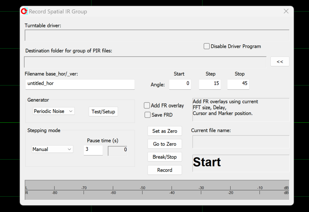
Using the Spacial impulse response group record function in Arta, you set the start and stop angle and increments and the software the simply steps you through each measurement automatically saving a PIR file each time.  All you need to do is make sure your measurement setup is correct in ARTA and the levels are ready to roll.

Close Mic measurements

Due to the gating that will be applied to our in room microphone measurements, we won’t have a picture of the real low frequency response of the speaker to build the crossover.  That leaves a pretty big risk of getting that low end correct in the final product, and as a bass aficionado that’s simply unacceptable.  To fix this, the common practice is to capture measurements of the woofer cone and port output directly and merge them together with these distance measurements to complete the picture.  So we have a couple more data points to capture before we move into Vituix to do the design work.

First, place the microphone within a few mm of the center of the cone of the woofer to capture the response.  This will require some level adjusting to not overload the microphone, which will be adjusted for when you process the files.  Run a single sweep in ARTA and save the output as an FRD file with phase.

Next, do the same thing at the same level for the port output.  I found that microphone placement was pretty critical and heavily affected the final levels.  The measurement guidance online indicated that the mic should be at about the plane of the port exit.  With a heavily tapered port like the Precision Port assembly I’m using, that plane is a little variable and the mic should be just inside the start of the taper.  This was pretty subjective, so in the end I’m not 100% confident in the port + woofer levels down under 50Hz where the port is important, but we’re close enough to concentrate on the crossover.

For this design it could be argued that the midrange also needed this close mic treatment, since that part of the cabinet is large and that little 4” mid will easily work to under 100Hz in that box.  However, I skipped this part based on the fact that the crossover between woofer and midrange will land near 500Hz, well above my expected 350Hz measurement limit.

Measurement Processing

With a stack of measurement PIR files, you’re ready to process them in Vituix.  This is done using the Convert IR to FR tool.

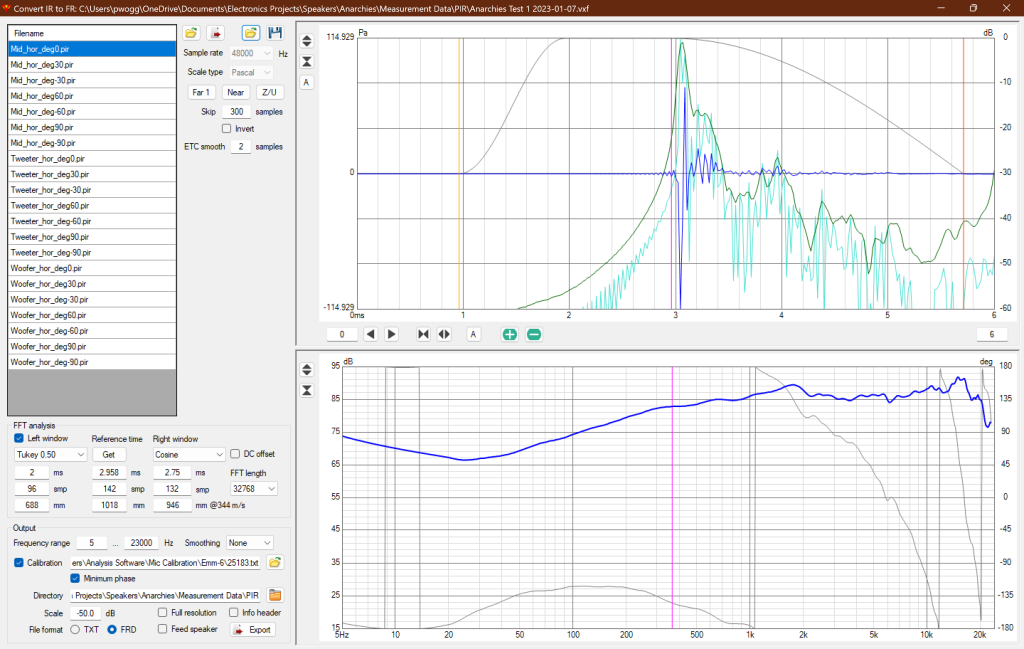
This tool with automatically run through all selected files with the same processing settings and spit out the resulting response files already named to match the input files.

With some online discussion help, the best gating settings were picked as a cosine window timed just under 3ms.  That gets my low frequency limit under 400Hz, but not quite to 300.

Close Mic Measurement Merging

Using another important tool in Vituix, we can take all the polar measurements we just processed and add the close mic woofer and port measurements taken to complete the low frequency picture of the finished speaker.

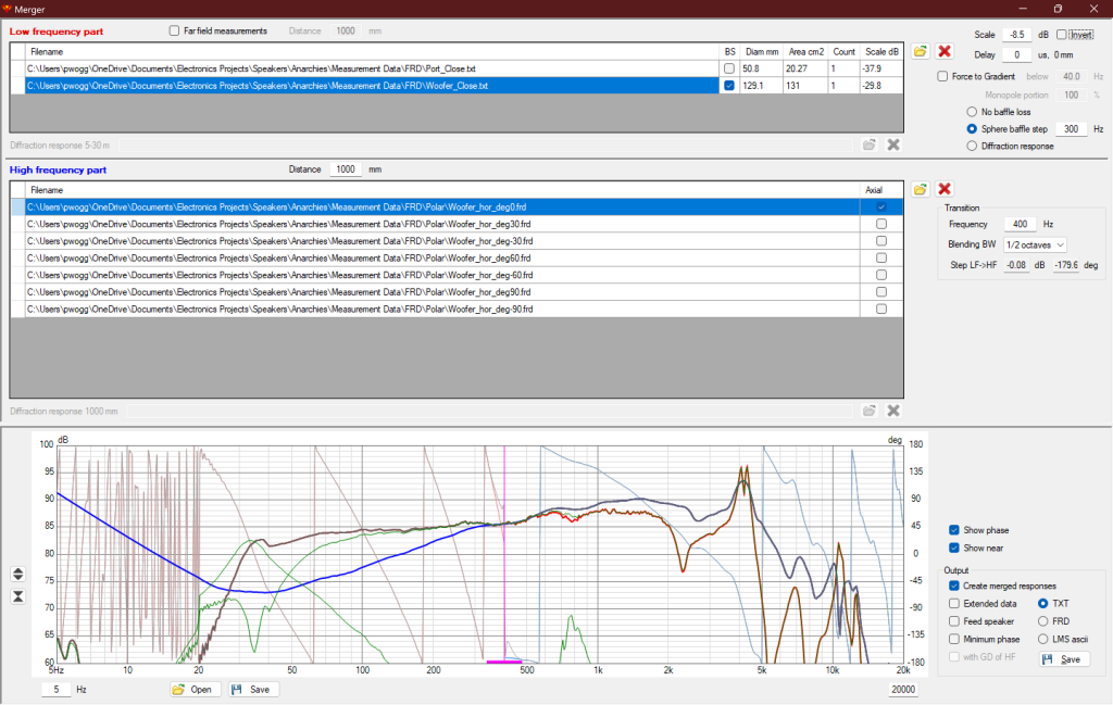
The close mic measurement files are loaded in the low frequency top section of the screen, with all the distance measurements loaded at the same time in the high frequency lower part of the screen.  There are a couple key settings on here to use in order to make your merged files as accurate as they can be.

First, the close mic measurement levels are relative to the radiating diameter of what you’re measuring.  So for the microphone the port close mic measurement will appear to be much higher SPL relative to the woofer cone due to the smaller radiating surface.  Vituix has you covered here, enter the diameter or area of the woofer and port and the SPL difference will be calculated and adjusted. 

Next, apply baffle step to the woofer by selecting Sphere Baffle Step when the woofer measurement is selected.  This will have a significant effect around 300Hz where your merge will land, the frequency is not likely exactly 300 as set based on the width of your baffle but it should be in that neighborhood.  Ultimately, changing the frequency has a minor effect relative to just turning it on and off so the end results won’t suffer much if you don’t accurately calculate and enter the frequency.

The merge frequency setting should be verified to be around or above the frequency limit of your gated measurements.

Finally, the Scale setting needs to be manually adjusted so the far field high frequency measurement level aligns with the low frequency parts where the merge is happening.  Just update that scale dB setting until the charts line up and blend smoothly.

Set your output to FRD and save!  Note, the minimum phase setting isn’t needed here since I used 2 channel measurements.  The phase data will be intact in the output files and minimum phase processing would lose that timing reference needed for later.

Crossover Design

Finally, we have the data required to really start digging into the filter design using Vituix.  There are many ways to start here, essentially the program loads with a clean slate so you’ll need to start out by:

• Defining your drivers on the Drivers tab
• Wiring them up with filters on the Crossover tab

Driver setup

On the Drivers tab, you’ll setup all the drivers used in the design and assign the frequency responses, impedance, and relative positions of everything so the simulation can be completed accurately.

For each driver, name them appropriately and define the settings on the screen.

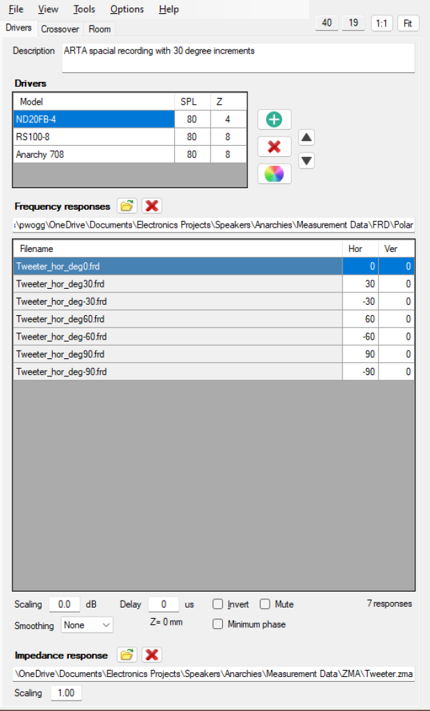
This includes loading all of the polar measurement data FRD files you’ve created.  As long as the naming convention is followed as it was setup by default through ARTA and the PIR processing, Vituix will know what to do with the measurement data. Don’t forget to load the actual impedance data in the box as measured by DATS or whatever tool you used in the format of a ZMA file.

Lastly for each driver, enter the X and Y offset data relative to the speaker on the design axis, usually the tweeter.  The Z information is not needed when you’ve used 2 channel measurements for the whole process, but the X and Y information is used to calculate the polar and power responses for the system so that bit is important.

Filter Creation

With the drivers defined, it’s time to wire them up.  There are many ways to do this, with some design tools like WinPCD helping you out with pre-created typical topology for the schematic.  In my case, I’m quite familiar with parallel passive filters so I was able to directly draw up 2^nd order filters for all drivers and begin to play with modifications to achieve my goals.

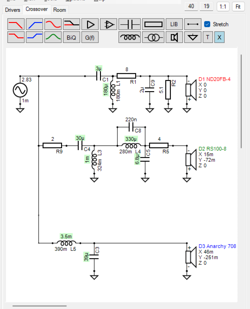
This is the final schematic for the design, but it took a little while to get here.  That part was some trial and error with the choices made based on basic RLC electronics theory.  I’ll explain some of the bits in detail.

Tweeter Network

This is a simple 2^nd order with an L pad + one extra capacitor to shape the high frequencies.  The components C1 and L1 make up the second order high pass filter.  Resistors R1 and R2 make up an L-Pad that attenuates the tweeter level to match the rest of the speaker.  Finally, C9 was added and when combined with the series resistor R1 in the L pad makes a first order low pass filter with a critical frequency at around 10kHz.  That critical frequency is calculated by the textbook formula 1/(2*pi*R*C) and defines the -3dB point of the filter.  What that does in the final response is attenuate the tweeter by 3dB starting at 10k with approximately 6dB per octave drop above that.  That’s the theory ignoring the parallel effect of R2 and the speaker itself. In reality the final effect is driven by those parallel elements and the actual in air frequency response of the tweeter as measured, so the real test is the final output response modeled.

Midrange Network

For the midrange, we have a set of 2^nd order filters for high pass and low pass plus two resistors for attenuation and phase alignment, and a single cap across the series coil making a tank notch filter in the circuit.  The components C4 and L3 make up the high pass filter while L4 and C5 make up the low pass filter.  The capacitor C8 was added across L4 to make a tank filter, the resonant frequency calculated by 1/(2*pi*SQRT(L*C)).  That places that notch up at 3.35kHz, right near the mid to tweeter crossover range.  Typically this is done in speaker filters to kill a nasty breakup frequency in the woofer, but in this case the RS100 doesn’t really have that problem. Instead, I made this addition based on the summation of the mid and tweeter at the crossover frequency.  Essentially, you want your summed output to be above the individual driver levels which indicates that the driver phases are reasonably in line and adding instead of subtracting.  Without that notch, this was not the case and was pointing to a phase alignment problem in that region.  The notch effectively increased the slope of the roll off of the midrange, allowing the drivers to add together more effectively. Finally, the resistors R9 and R5 are in there to reduce the midrange level to meet up with the woofer, which is always the gating factor for final speaker sensitivity and bass output.

Woofer Network

For the woofer I’ve only used the 2 components L5 and C3 to make up a simple 2^nd order low pass.  During design iterations, I did play with more complicated networks including adding a RC Zobel in parallel to the woofer in an attempt to shape the filter slope, but in the end this proved to not improve anything with the system response and was removed to save final cost.

Comparison between Variants

Vituix has some really handy tools to save, recall and compare different tweaks to values in the same file to allow easy changes and comparisons for the final output.

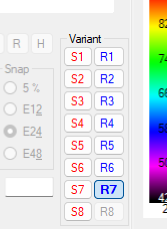
The little variant section on the screen allows you to store changes by simply clicking the S1 through S8 buttons.  To compare, simply click the R1 to R8 buttons to instantly switch between crossovers.

The Optimizer

This super handy tool in Vituix is not super well documented.  I made many attempts using it and watched as the tool simply iterated 500 times and resulted in a much worse output than I had done myself manually.  It turns out there are some very important steps before using this tool to make it work properly, and once you do it can help your design become as good as possible for your goals.

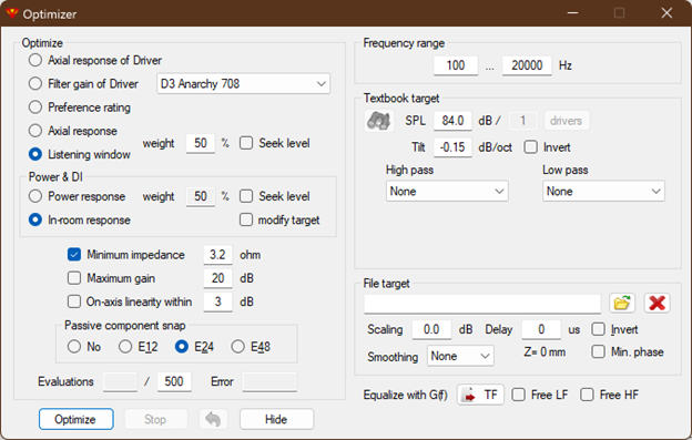
The optimizer window is where you’ll start to get it setup.  For my design goals, I’m optimizing for in room power response and listening window response with 50% weight on either.  That means the goal will be smooth across a small horizontal angle instead of only on axis, and the in room calculated response will be calculated as equally important.  I also set a minimum impedance here and set the component values to snap to standards to improve the chance of actually being able to buy the final values.

On the right side of the optimizer screen, we have some very important settings to make in order for the optimization to work.  This part had to be pointed out to me, and I didn’t see or catch this in the documentation.  In order for the iterations to work, you must properly set the target to work toward!  This must be realistically achievable by limiting the frequency range, or the system will simply iterate and give up.  You also want to land the target SPL correctly or it won’t be able to hit that either.

For this design I have a slight downward slope of -0.15dB per octave across a wide target range of 100Hz to 20kHz.

Then back on the schematic screen, you have to tell Vituix which components it should alter to meet that optimization target.   The tool works best on the standard crossover blocks for the high pass and low pass elements as well as the regular L-Pad and attenuation resistors, so skip the extra parts like the extra capacitors added for the tank and tweeter contour capacitor.  Right click on your components and turn on optimize to let it do its thing.  Run the tool and watch how the output graph changes, then play around and run it some more.

Trial and Error

At this point, you’re into just tweaking things a bit here and there until you’re happy with the output results.  After optimization, tweak your extra parts to see what happens, adjust things, keep saving variants and comparing.

Interpreting the Output

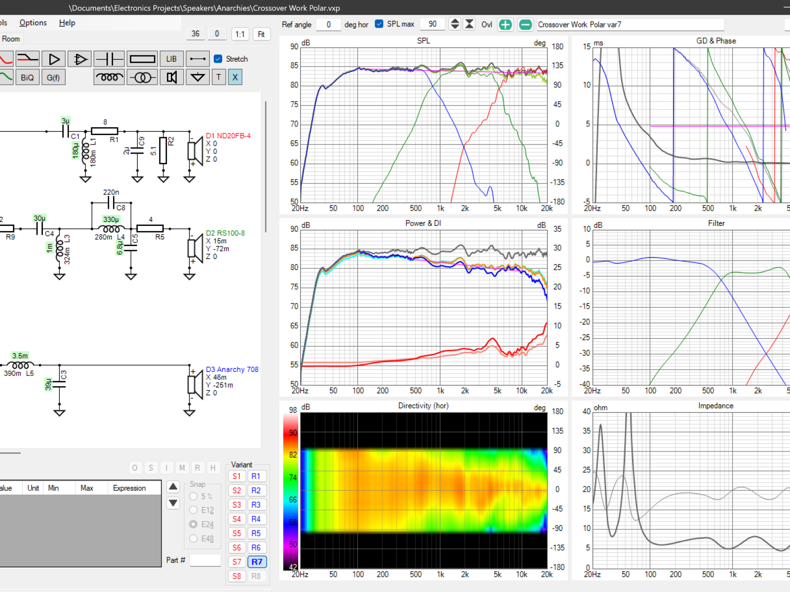
The output in Vituix that will tell you how your speaker will perform in real life is all part of what they call the 6 pack.

SPL

This chart is the resulting output response of the whole system, showing the individual driver outputs and how they sum up on axis and across the listening window.  Your target is also displayed, allowing you to see how close to ideal you’ve come.   This is where you want as straight of a line as possible for the final product, and in line with your target.

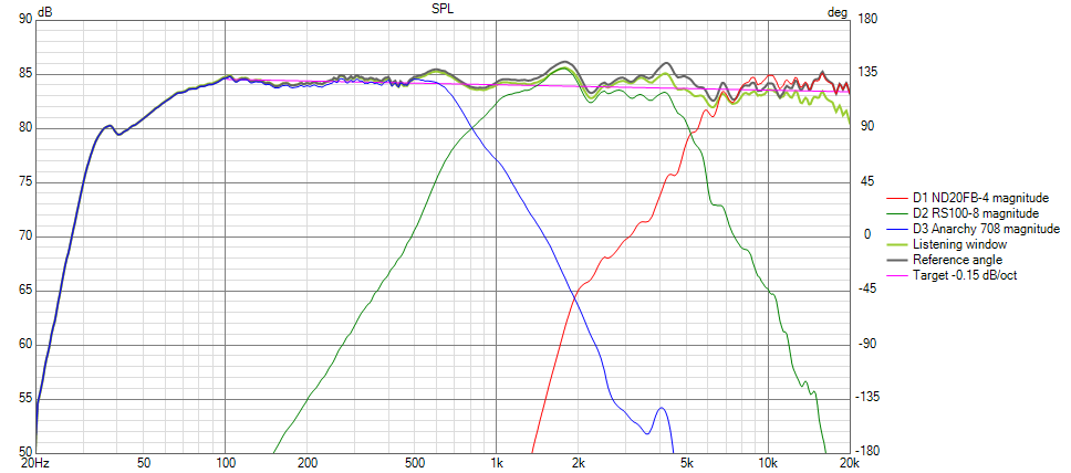
The simulation result here shows the target right in the middle of the final results and within a couple dB ether way.

Power & DI

This chart shows you the room response predicted at the simulation distance, which defaults to 2.5 meters away from the speaker.  That’s about right for my listening room, so that’s what I stuck with.

The goal here is to have the in room, ER and Power Response all as smooth as possible.  Speakers will often bunch up with a rise in power response where the tweeter takes over from the midrange.  This is caused by the change in dispersion when the transition from a large diameter woofer to a small diameter tweeter happens.  While this is a law of physics based on diameter of a radiating surface so it cannot be completely controlled, the filter can influence the transition enough to smooth the final output.

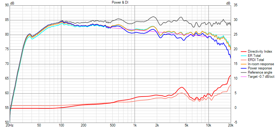
The simulation results here show the power response curves are now similar to the reference angle.  The prediction is that the room response is just as smooth as it tilts down naturally and does not have any undue rise in response as the drivers transition to each other.  The directivity lines at the bottom would ideally be straighter, and there is a slight lump as the tweeter takes over as we fight the laws of physics.  This is really typical, and pretty good for reality.

Directivity

This chart visualizes how the speaker output changes off axis.  There are several display options for this, the heat map being the default display.  With the heat map, you can see where things may be hot or cool off axis.  The final goal is to be as smooth as possible with little to no large changes in output off axis beyond the expected roll off.

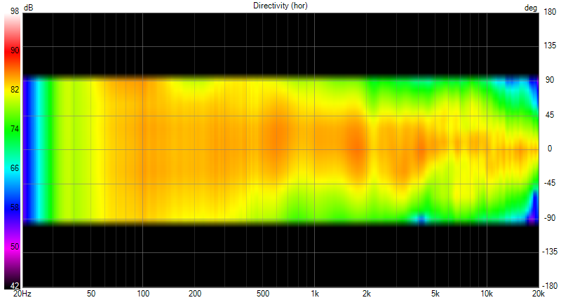
This simulation results shows a pretty smooth off axis distribution.  Note the slight tilt to the orange parts of the spectrum.  This is due to the asymmetric angle to the baffle and driver mounting positions and is expected.  Once both complementary speakers are built, I expect the tilt of these measurements to be complementary as well.

Note the limit of the chart at 90 degrees is due to my choice of limiting the spin-o-rama measurements to that angle. Continuing to measure all the way around the speaker will complete the rest of this chart.

GD & Phase

This chart shows the phase of the individual drivers as well as the full system and shows you the group delay expected as well.  This is useful for ensuring that the phase between drivers are aligning at the simulation point.  This wasn’t a priority for the design since the focus was on and off axis smoothness in the final summed output.  The phases simply needed to be close enough to allow efficient summation as the drivers crossed over.

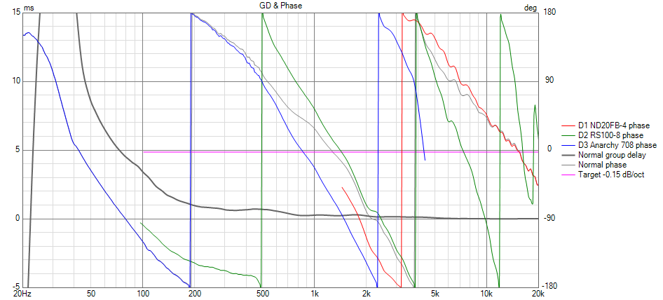
Not much to note in this simulation output.  You can see the tweeter and midrange are not quite in phase alignment or the red and green traces would be on top of each other.  In this case, they’re within about 30 degrees, which is plenty close to avoid being destructive when adding together in the air.

Filter

This chart shows the transfer functions of the filter itself, allowing you to see what and how much attenuation you have for each driver and the shape you’re applying electrically.  There is no goal here, just information.

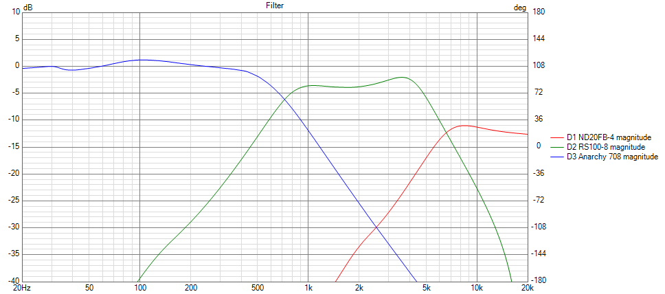
The filter output here shows the levels of attenuation needed on the mid and tweeter to bring them into alignment.  Note the tweeter is about 11dB down from the woofer level, so it will receive less than 1/10^th the power of the woofer to generate the same SPL.  You can also see the downward slope introduced by using the low pass capacitor C9.

Impedance

This last chart is quite important for the amplifier you intend to hook your speaker to.  All amplifiers have a minimum impedance they can handle with consumer amplifiers being setup for 8 ohm nominal.  That’s a classic misunderstanding in speakers, 8 ohm does NOT mean 8 ohm in reality and instead means that the speaker is somewhere around 8 ohms for much of its frequency range.

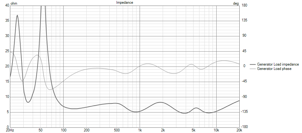
An 8 ohm nominal speaker can easily be in the 6 ohm range at DC, and amplifiers generally have no problem driving a lower load within reason.  The results here show the speaker spending a lot of time in that 5 ohm range without large swings in impedance that translate to heavy phase angles.  This will be a bit of a challenge for a cheaper consumer amplifier, but not too terrible.  In the end, I would call this a 6 ohm nominal speaker rather than 8.

Preparing to Build

After finally settling on the simulation I liked, it was time to gather all parts for build.  I did this with a little evaluation of the parts I had on hand and what was needed to order.

Vituix List			Available
RefDes	Value	DCR / ESR / P	Actual	DCR	Part Number	Cost	Qty	On Hand	Net
L1	180 μH	0.22 Ω	0.18 mH	0.18	255-208	$            7.55	2		$             15.10
L3	1 mH	0.324 Ω	1 mH		N/A	$                –	2	2	$                   –
L4	360 μH	0.325 Ω	0.33 mH	0.28	N/A	$                –	2	2	$                   –
L5	3.6 mH	0.374 Ω	3.5 mH	0.39	257-560	$            8.59	2		$             17.18
C1	3 μF	10 mΩ	3 uF		027-220	$            3.95	2		$               7.90
C3	39 μF	10 mΩ	39 uF		N/A	$                –	2	2	$                   –
C4	30 μF	10 mΩ	30 uF		027-258	$         21.98	2		$             43.96
C5	6.8 μF	10 mΩ	6.8 uF		027-238	$            6.15	2		$             12.30
C8	220 nF	10 mΩ	0.22 uF		N/A	$                –	2	2	$                   –
C9	2 μF	10 mΩ	2 uF		027-214	$            2.86	2		$               5.72
R1	8 Ω	10 W	8 ohm		N/A	$                –	2	2	$                   –
R2	5.1 Ω	10 W	5.1 ohm		004-5.1	$            1.49	2		$               2.98
R5	4 Ω	5 W	4 ohm		N/A	$                –	2	2	$                   –
R9	2 Ω	5 W	2 ohm		N/A	$                –	2	2	$                   –
									$           105.14

Then it was time to work on the final finish of the cabinets and gather the parts to make this all in reality.